How do you handle high-throughput, schema-less updates and make that same data queryable at scale?

Recently, our team hit a technical wall when we set out to build a new feature that enables customers to write, persist, and query user-level properties on our servers. Namely, “How do you handle high-throughput, schema-less updates and make that same data queryable at scale?”

If you’re familiar with Google Cloud, you know that Bigtable is designed for the former use case: ingesting data flexibly at scale. BigQuery lets you do, well, big queries, but it requires the data you’re analyzing to be highly structured. Getting the best of both worlds in GCP native was not an option out-of-the box, so we made our own solution.

In this post, we’ll walk through how we solved this by replicating Bigtable updates into a Type 2 SCD (Slowly Changing Dimension) model in BigQuery. Part of our solution involved joining GCP’s private preview of fine-grained DML to make it all work affordably at scale.

The problem

At Statsig, we build tools for B2B product analytics, event logging, experiments, and feature management. Behind the scenes, that means ingesting a huge firehose of user events, metrics, and property updates (up to hundreds of thousands per second). We also have to process this data to be queryable so customers can view and analyze user behavior in dashboards, graphs, and more.

The main challenge was that we needed to enable schema-less read/write point operations at scale while still allowing for near real-time, large analytical queries. The problem space and constraints in detail were as follows:

1. Customers send a large volume of user-property updates, typically with our SDKs. We need to be able to store and retrieve these updates at scale, with single-digit-millisecond latency.

2. The user-property updates are schema-less and come in all sorts of shapes, sizes, and forms since they are coming from all types of customers/companies. The way we ingest this data needs to be flexible.

3. We also need to store these updates in a versioned manner since customers often want to observe how user behavior changes over time or with different properties. For example, “How does user behavior on our app change before, during, and after they obtain a premium subscription?”

4. Customers need to be able to do whole table, large analytical queries on this user-level data, such as for building user metric dashboards.

Solution overview

At a high-level, our solution works by replicating the user-property updates in Bigtable into a Type 2 SCD BigQuery table. Here’s how it works:

1. User-property updates are generated in one of two ways (in blue). Customers either set up bulk uploads in our web console, or they use our SDKS to log them at run-time.

2. We have a User Store Service that sits in front of Bigtable (in orange). It handles ingesting user-property updates from either source and just focuses on getting all the data in, without dropping anything.

3. We have Bigtable set up with CDC enabled (in pink). This is what we use to track and replicate changes made to user properties in Bigtable.

4. Then, we have a Dataflow that reads those updates from Bigtable CDC, and streams those to BigQuery in near real-time.

5. Finaly, we have a scheduled BigQuery job that materializes this CDC data into the Type 2 SCD table in its queryable “final form” so that it’s ready for customer analytics use cases (in green).

In summary, Bigtable delivers the speed and schema flexibility needed for the ingestion, whereas BigQuery delivers the horsepower for large scans and joins. By streaming Bigtable Change Data Capture (CDC) into a Type 2 SCD table, we merged the two systems into a single, consistent view of current and historical data.

Solution deep-dive

Part 1: Bigtable

Bigtable is great for the first part of our solution because it lets user properties live in a dedicated column family without a pre-defined schema. This allows us to store thousands of arbitrary user properties per user in a very flexible manner, as not all columns have to be filled. This is important because we service a wide variety of industries and customers, and one company’s “user” schema can be wildly different from another.

Bigtable’s write path also comfortably sustains millions of QPS, so cross‑region replication keeps read latency below 10 ms no matter wherever the request originates, letting us replicate it in near real-time.

Finally, to capture every update and allow for user-property “version history”, we enabled Change Streams in Bigtable. This emits an ordered log of cell changes that includes both the commit_timestamp and a monotonic tiebreaker. This feed becomes the authoritative record of how any property evolved.

Part 2: Dataflow

The next part was to actually enable streaming data from the Bigtable to BigQuery. We used Google’s Bigtable‑to‑BigQuery streaming template to consume the Change Stream and insert each event into a BigQuery changelog table. The template handles ordering guarantees, retries, and watermark advancement, so our pipeline code remains minimal. End‑to‑end latency from a Bigtable write to BigQuery is typically two to three minutes, which enables customers to create near real-time analytics dashboards and alerting.

Part 3: BigQuery and the Type 2 SCD approach

As you might guess, the raw changelog from this streaming template grows really fast. To address this, in the replication process to BigQuery, we have a scheduled MERGE statement that transforms the giant changelog into a nice, materialized SCD Type2 table. It keeps the latest version of each property marked as “current” while retaining every prior version.

This table is partitioned based on the date it becomes inactive and clustered on row_key, property_key, and big_query_commit_timestamp. This allows us to efficiently rebuild what the table looked like at some point and time as well as quickly determine the current state of active rows.

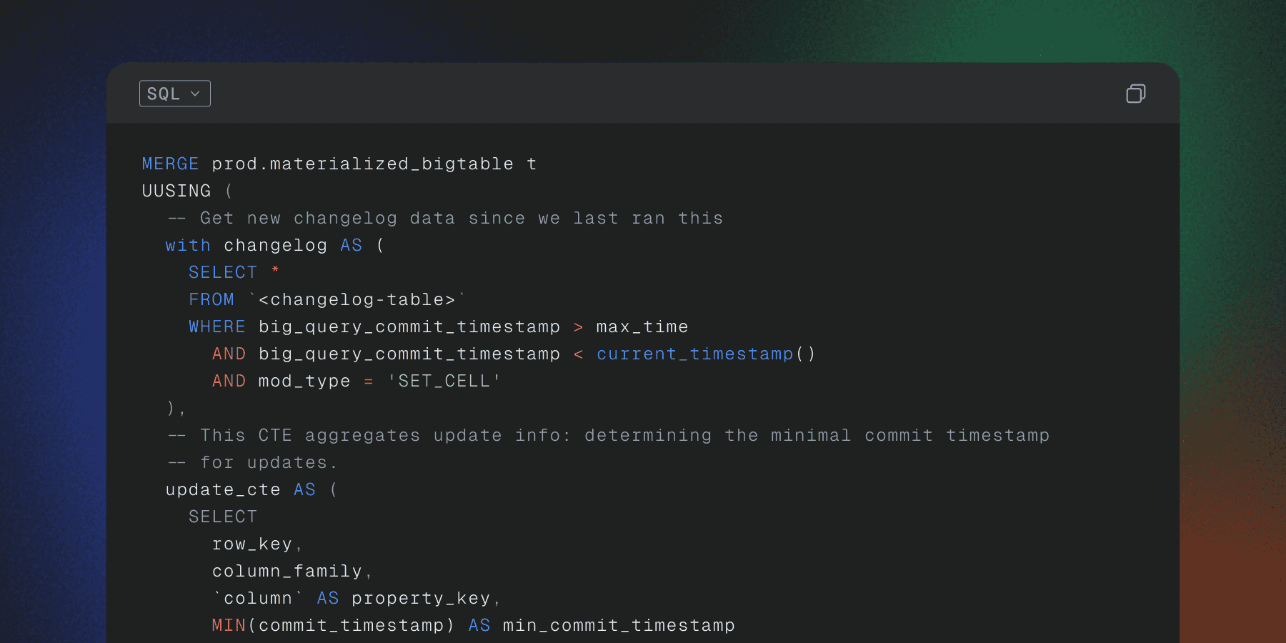
Here is an example of how we merge new changelog data into the existing table. This query only supports inserts and updates, not deletes:

MERGE prod.materialized_bigtable t
USING (
  -- Get new changelog data since we last ran this
  WITH changelog AS (
    SELECT * FROM `<changelog-table>`
    WHERE big_query_commit_timestamp > max_time
      AND big_query_commit_timestamp < current_timestamp()
      AND mod_type = 'SET_CELL'
  ),
  -- This CTE aggregates update info
  update_cte AS (
    SELECT
      row_key,
      column_family,
      `column` AS property_key,
      MIN(commit_timestamp) AS min_commit_timestamp
    FROM changelog
    GROUP BY row_key, column_family, property_key
  ),
  -- This CTE prepares new rows to be inserted
  insert_cte AS (
    SELECT
      row_key,
      column_family,
      `column` AS property_key,
      value AS property_value,
      commit_timestamp,
      tiebreaker,
      LEAD(commit_timestamp) OVER (
        PARTITION BY row_key, column_family, `column`
        ORDER BY commit_timestamp, tiebreaker
      ) AS current_until_timestamp,
      big_query_commit_timestamp,
      IF(
        LEAD(commit_timestamp) OVER (
          PARTITION BY row_key, column_family, `column`
          ORDER BY commit_timestamp, tiebreaker
        ) IS NULL, TRUE, FALSE
      ) AS is_current
    FROM changelog
  )
  SELECT 
    u.row_key,
    u.column_family,
    u.property_key,
    NULL AS property_value,
    NULL AS commit_timestamp,
    NULL AS tiebreaker,
    u.min_commit_timestamp AS current_until_timestamp,
    NULL AS big_query_commit_timestamp,
    NULL AS is_current,
    TRUE AS is_merge_update
  FROM update_cte u
  UNION ALL
  SELECT 
    i.row_key,
    i.column_family,
    i.property_key,
    i.property_value,
    i.commit_timestamp,
    i.tiebreaker,
    i.current_until_timestamp,
    i.big_query_commit_timestamp,
    i.is_current,
    FALSE AS is_merge_update
  FROM insert_cte i
) AS src
ON 
   src.is_merge_update = TRUE  
   AND target.is_current
   AND target.row_key = src.row_key
   AND target.column_family = src.column_family
   AND target.property_key = src.property_key
WHEN MATCHED AND target.is_current = TRUE THEN
  UPDATE SET target.is_current = FALSE,
             target.current_until_timestamp = src.current_until_timestamp
WHEN NOT MATCHED THEN
  INSERT ( row_key, column_family, property_key,
           property_value, commit_timestamp, tiebreaker, current_until_timestamp,
           big_query_commit_timestamp, is_current )
  VALUES ( src.row_key, src.column_family,
           src.property_key, src.property_value, src.commit_timestamp, src.tiebreaker,
           src.current_until_timestamp, src.big_query_commit_timestamp, src.is_current );

Part 4: Fine‑grained DML

Another piece of our solution was fine-grained DML, which lets us do more efficient and granular edits than with traditional BigQuery DML. With this, BigQuery is able to batch mutations periodically instead of needing to do them for every query. For queries that run often and make large amounts of mutations, this drastically lowers the cost of performing updates/deletes.

In our case, we were spending several hundreds of dollars a day on this part of our architecture, but getting access dropped the slot cost of running this query by over 6X while maintaining fast read performance.

Fine-grained DML in BigQuery is currently still in private preview, but we were able to get in on this with the help of some of our friends at GCP (shoutout to Keane and Alex). If you’re interested in it, check out their docs.

SCD Query Examples

The resulting table in BigQuery is very flexible. Here are some examples of how we query the data that lives in Bigtable, but using BigQuery.

1. The current state of the Bigtable:

SELECT *
FROM prod.user_store_materialized
WHERE is_current;

2. The state of the Bigtable at some moment in time:

SELECT *
FROM prod.user_store_materialized
WHERE rowkey = @rowkey
  AND @as_of BETWEEN commit_timestamp
                AND COALESCE(current_until_timestamp,
                              TIMESTAMP '9999-12-31');

3. How some property has changed over time:

SELECT commit_timestamp, property_value
FROM prod.user_store_materialized
WHERE rowkey = @rowkey
  AND property_key = '<some_property>'
ORDER BY commit_timestamp;

Partition pruning on current_until_timestamp plus clustering on the rowkeys keeps these scans tight, even as history piles up.

This was a feature that we wanted to unlock for our cloud customers for quite a while now. While we’re not the first company to offer it, our implementation is unique and cost-efficient. Some competitors allow customers to query a user’s properties at their first vs. last sessions; others do store and query such data, but with slow performance. Technically speaking, our implementation could enable fast querying of all versions of a user.

In summary, Bigtable supplies the low‑latency, schema‑flexible storage for live user properties and a managed Dataflow template. By streaming every mutation into BigQuery using a Type 2 SCD table (and maintaining costs with Fine‑grained DML), we were able to support both the current operational view and deep historical analysis. It all lives in one pipeline, two workload classes, and zero duplicate write paths.

We took a lot of inspiration from this blog on Efficient Management of SCD Type 2 Tables for Machine Learning and Big Data and wrote this up for anyone else in the community looking to create a similar solution. If you’re interested in other cool engineering problems we’re solving at Statsig, check out the rest of our engineering blogs.

Looking for a smarter way to ship?

Statsig combines enterprise-grade feature flags with your product metrics, helping you ship fast, without breaking things

Book a demo now